Big-O Notation: A Refresher
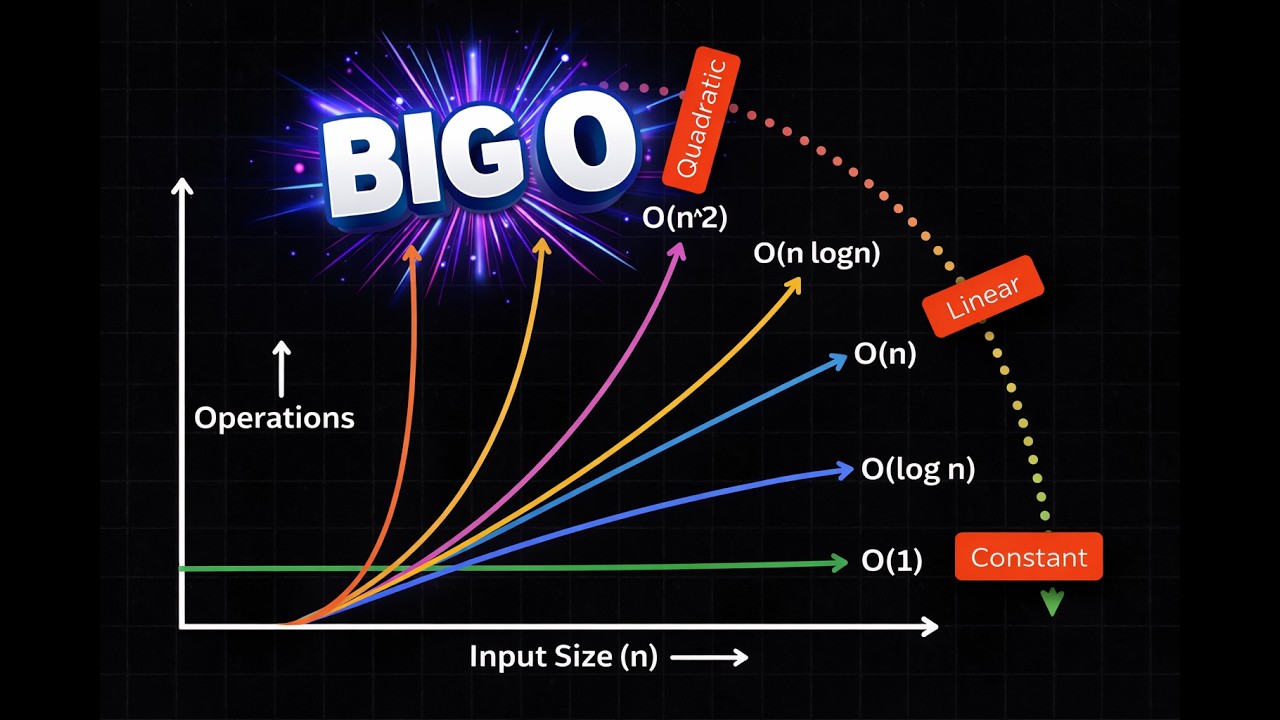
Big-O notation is a fundamental concept in computer science that helps us understand the efficiency of algorithms and data structures. It gives us a language to analyse and compare the performance of different algorithms based on input size – without getting bogged down in hardware details or constant factors.
Despite reading books, watching videos, and implementing algorithms, Big-O notation is one of those topics that never properly stuck in my head.
So I decided to take some time to revisit it and finally make it click.
This post pulls together the explanations that helped me most: a Red Gate blog post from around May 2020 (with the accompanying repo maceage/tackle-big-o-net-core), NeetCode’s Big-O Notation for Coding Interviews and Big-O Notation – Everything you Need for Coding Interviews, plus Fireship’s Big-O Notation in 100 Seconds video.
There is also the Big-O Algorithm Complexity Cheat Sheet that shows common data structure operations and array sorting algorithms that can be referenced in a pinch.
Painting a Fence
One example that made things click for me was the painting-a-fence analogy. The total work depends on three independent factors:
Painting a fence = O(w · h · p)
where:
w= width in metresh= height in metresp= number of paint layers
If you double the width, you double the work. If you double both width and height, the work quadruples. That multiplicative intuition carries straight over to nested loops.
Drop the Non-Dominant Terms
When simplifying, keep only the term that grows fastest as N grows:
| Original | Simplified |
|---|---|
| O(N² + N) | O(N²) |
| O(N² + log N) | O(N²) |
| O(5·2ⁿ + 1000N¹⁰⁰) | O(2ⁿ) |
Constants vanish too: at scale, N² + 1000 and N² behave the same.
O(log N) Runtimes
Binary search halves the problem space each step:
N = 16
N = 8    // divide by 2
N = 4    // divide by 2
N = 2    // divide by 2
N = 1    // divide by 2
Running it in reverse doubles each time: 1 → 2 → 4 → 8 → 16.
Since 2⁴ = 16, we have log₂16 = 4 – that exponent is the number of halving steps.
Rule of thumb: if the number of elements in the problem space halves on each iteration, you probably have an O(log N) runtime. It’s also why finding an element in a balanced binary search tree is O(log N): each comparison discards half the remaining tree.
Adding vs. Multiplying Runtimes
Sequential loops add:
for (int a : arrA) {
    print(a);
}

for (int b : arrB) {
    print(b);
}

// O(A + B)
Nested loops multiply:
for (int a : arrA) {
    for (int b : arrB) {
        print(a + "," + b);
    }
}

// O(A * B)
Recursive Runtimes
Consider:
int f(int n) {
    if (n <= 1) {
        return 1;
    }

    return f(n - 1) + f(n - 1);
}
Each call spawns two more, producing a tree of calls:
                       f(4)
             f(3)               f(3)
        f(2)    f(2)       f(2)    f(2)
f(1)f(1) f(1)f(1) f(1)f(1) f(1)f(1)| Level | # Nodes | Expressed as |
|---|---|---|
| 0 | 1 | 2⁰ |
| 1 | 2 | 2¹ |
| 2 | 4 | 2² |
| 3 | 8 | 2³ |
The total node count is 2⁰ + 2¹ + 2² + ⋯ + 2ⁿ, a geometric series whose sum is roughly 2^(n+1) – so the runtime is O(2ⁿ).
Rule of thumb: a recursive function’s runtime is O(branchesᵈᵉᵖᵗʰ), where branches is the number of recursive calls each invocation makes.
Amortized Time
Consider a dynamic array (like C#’s ArrayList) that doubles its capacity when full:
- When capacity is hit, a new array is allocated and all N elements copied – O(N) for that single operation
- But the majority of insertions are O(1)
- X insertions in total cost about O(2X) work
Spread across many operations, that averages out to O(1) per insertion.
Amortized time = the average time per operation, measured over many operations – the long-run worst case, rather than any single unlucky operation.
Wrapping Up
Looking back over these notes, the thing that finally made Big-O stick wasn’t memorising a table of complexities – it was recognising a handful of shapes that keep showing up:
- Work that scales with every independent dimension → multiply the factors (the fence)
- Sequential work adds, nested work multiplies
- Halving the problem each step → logarithmic
- Recursive branching → exponential in the depth
- Occasional expensive operations spread thin enough to disappear → amortized
Almost every complexity I’ve bumped into since is some combination of those patterns, and being able to eyeball unfamiliar code and ask “which shape is this?” has been far more useful than recalling exact definitions.
The other lesson: sometimes a topic doesn’t land the first time, or even the third – and that’s fine. Leaving it alone for months and coming back with fresh material (a different video, a different analogy, some code you wrote yourself in between) is often all it takes for it to click.
If Big-O hasn’t stuck for you yet, I’d recommend picking whichever resource above matches how you learn best and giving it another pass – ideally with a whiteboard nearby.
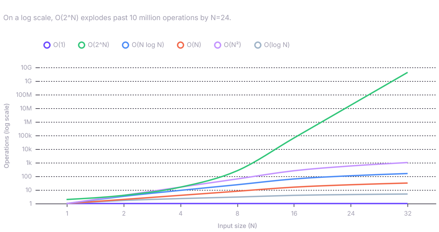
Complexity Comparison Chart
And here’s the growth-rates chart — note the logarithmic y-axis, since O(2ⁿ) would otherwise flatten everything else into a flat line at zero:
Related Posts
2024-08-30
2024-03-03